Do you want to buy antibiotics online without prescription? https://buyantibiotics24h.net/ - This is pharmacy online for you!
Www2.georgetown.edu
Journal of Biopharmaceutical Statistics, 18: 468–482, 2008Copyright Taylor & Francis Group, LLCISSN: 1054-3406 print/1520-5711 onlineDOI: 10.1080/10543400801993002
SAMPLE SIZE CALCULATIONS IN THOROUGHQT STUDIES
Lu Zhang1, Alex Dmitrienko1, and George Luta2 1Lilly Research Laboratories, Eli Lilly and Company, Indianapolis, USA 2Georgetown University, Washington, DC, USA An analysis of QTc data collected in four thorough QT studies conducted at Eli Lilly and Company was performed to estimate the variability of the QTc interval and to calculate the variance components related to time-to-time, day-to-day variability, etc. The results were used to develop a sample size calculation framework that enables clinical trial researchers to account for key features of their thorough QT studies, including study design (parallel and crossover designs), number of ECG replicates, number of post-baseline ECG recordings, and subject population (based on subject gender and age). The sample size calculation framework is illustrated using several popular study designs. Key Words:
QT interval; Sample size; Thorough QT study; Variability.
The assessment of cardiac liability of new compounds is becoming an
increasingly important component of preclinical and clinical drug development. The QT interval, which represents the duration of ventricular depolarization andsubsequent repolarization on a 12-lead electrocardiogram (ECG), is a commonlyused surrogate marker for life-threatening cardiovascular events (ventriculararrhythmias) in clinical trials.
The International Conference on Harmonization (ICH) published a guidance
document (ICH E14, 2005) to describe strategies for the evaluation of cardiacsafety of new drugs in clinical development. This document introduced a newapproach to the assessment of the proarrhythmic potential of new drugs (thoroughQT study). The objective of this study is “to determine whether the drug has athreshold pharmacologic effect on cardiac repolarization, as detected by QT/QTcprolongation” (ICH E14, 2005, Section 2.2). It is estimated that more than 50thorough QT studies have been conducted over the past five years, and about10 thorough QT study reports have appeared in medical journals, for a listof published thorough QT studies, see Biopharmaceutical Network’s Website(http://www.biopharmnet.com/doc/doc14001-01.html).
Received August 22, 2007; Accepted January 12, 2008Address correspondence to Alex Dmitrienko, Eli Lilly and Company, Lilly Corporate Center,
Indianapolis, IN 46285, USA; E-mail: dmitrienko_alex@lilly.com
SAMPLE SIZE CALCULATONS IN QT STUDIES
Since thorough QT studies have become a key component of clinical drug
development, they have attracted attention in the biostatistical literature. Mostof the papers in this area focus on the analysis of data collected in thoroughQT studies. This includes general analysis approaches (Patterson et al., 2005), QTcorrections for heart rate (Dmitrienko and Smith, 2003; Ma et al., 2008), andmultiplicity issues (Boos et al., 2007; Eaton et al., 2006). This paper focuses on thedesign of thorough QT studies and discusses sample size and power calculations.
Eli Lilly and Company has recently conducted four thorough QT studies.
The QTc data from these studies were analyzed to estimate the variability of theQTc interval and calculate the variance components related to minute-to-minute,day-to-day variability, etc. The results were used to develop a general approach toperforming sample size calculations for thorough QT studies that is applicable to abroad range of trial designs.
This paper is organized as follows: Section 2 describes the four thorough
QT studies included in the analysis of the QTc interval. Section 3 discusses themodeling approach used in the estimation of variance components and summarizesthe results of the pooled analysis. Section 4 summarizes key considerations in samplesize calculations in the context of thorough QT studies, and Sections 5 and 6discuss methods for computing sample size and power in thorough QT studieswith crossover and parallel group designs. Sections 5 and 6 also give examples andreview guidelines for sample size calculations in designs widely used in thorough QTstudies.
An analysis of QTc interval measurements was performed using 12-lead ECG
data collected in four thorough QT studies recently conducted at Eli Lilly andCompany. The studies were conducted to evaluate the effect of a test drug on theQTc interval compared to placebo in healthy subjects. The ECG data were collectedusing the same process across the four studies. The process included the followingcomponents:
• ECG recordings were captured using standardized digital equipment.
• A standardized algorithm was utilized to measure QT intervals.
• ECG recordings were overread by a single cardiologist in each study who used
standardized ECG interpretation guidelines.
• Standardized data edits were applied to ensure the quality of the ECG data.
The consistency of the ECG collection and management processes across the studiesserved as a justification for the combined analysis of QT interval and heart ratemeasurements across the studies.
A brief description of the individual studies is given below and a summary of
subject characteristics is displayed in Table 1.
Study 1 (Beasley et al., 2005) was a three-period crossover study with three
treatments, tadalafil, placebo, and ibutilide (positive control). There were twolead-in days at the beginning of each period and five to six ECG recordings weretaken during the lead-in and dosing days. Ten replicate ECGs were collected at eachscheduled time point. ZHANG ET AL.
characteristics in four thorough QT studies
Study 2 (Zhang et al., 2007) was a three-period crossover study with three
treatments, duloxetine, placebo, and moxifloxacin (positive control). There wasone lead-in day at the beginning of the trial. The duloxetine and placebo periodsincluded a four-day dose escalation scheme with four doses, and four ECGrecordings were taken on the fourth dosing day of the two highest levels. Fourreplicate ECGs were collected at each scheduled time point.
Study 3 (unpublished) was a three-period crossover study with three
treatments, experimental drug, placebo, and moxifloxacin (positive control). Therewas one lead-in day at the beginning of the study, and three ECG recordings weretaken during the lead-in and dosing days. Four replicate ECGs were collected ateach scheduled time point.
Study 4 (unpublished) was a three-period crossover study with three
treatments, experimental drug, placebo, and moxifloxacin (positive control). Therewas one lead-in day at the beginning of the study, and three ECG recordings weretaken during the lead-in and dosing days. Four replicate ECGs were collected ateach scheduled time point.
The main objective of the analysis of QTc measurements was the estimation of
variance components related to the random subject effect and random effects relatedto multiple days within each treatment period and multiple time points (at whichECG recordings were taken) within each day. This information was used to supportsample size calculations for important types of thorough QT studies (see Sections 5and 6).
The analysis focused on the QT interval corrected for heart rate using the
Fridericia correction or QTcF (Fridericia, 1920). The Fridericia correction waschosen because it is currently the most popular QT correction approach in thoroughQT studies. The analysis included 34,913 drug-free ECG recordings collected in thefour studies described in Section 2 (26,721 ECG recordings from Study 1; 4869ECG recordings from Study 2; 1883 ECG recordings from Study 3; and 1440 ECGrecordings from Study 4).
In order to estimate the variance components, it was assumed that serial
QTcF measurements for each subject follow a multivariate normal distributionand QTcF measurements within each day are equicorrelated. The assumption ofmultivariate normality has been confirmed in multiple studies (Patterson et al.,
SAMPLE SIZE CALCULATONS IN QT STUDIES
2005), and the assumption of equicorrelated measurements is commonly made tosimplify theoretical calculations (Boos et al., 2007). A multivariate model with thiscovariance structure provides a reasonably good fit to QTcF data and, althoughthe fit can be improved by adding random terms with an autoregressive covariancestructure, the magnitude of this improvement is rather small.
Mixed-effect models with normally distributed random effects were fitted to
serial QTcF measurements from drug-free ECG recordings collected in the fourthorough QT studies. Let X
denote the QTcF measurement for the ith subject on
the jth day at the kth time point obtained from the lth replicate ECG. The followingmodel was assumed:
Here D and T are fixed effects corresponding to the day and time. Further,
are random effects for the subject and related interactions (subject-by-
day, subject-by-time, and subject-by-day-by-time) with standard deviations
is the residual term with standard deviation
Mixed-effect models of this kind can be used to approximate covariance structuresin a variety of designs encountered in thorough QT studies, including complexcrossover designs with multiple lead-in days in each treatment period.
Standard deviations of the variance components included in the mixed-effect
models were estimated in each thorough QT study, and a pooled analysis of thefour studies was also performed. In addition, similar analyses, with random-effectcontrasts between gender groups or age groups in the model, were performed forkey demographic subgroups (males, females, and subjects younger and older than50 years). The results (standard deviations of individual variance components andassociated standard errors) are displayed in Tables 2 and 3.
Table 2 summarizes the results of the study-specific and pooled analyses.
Although there is a certain degree of study-to-study variation, the variabilityestimates are generally quite consistent across the four thorough QT studies. Theestimated variance components range from 9.69 to 13.75 ms for the subject term,
Table 2 Variance components for the Fridericia-corrected QT interval estimated from drug-free ECG recordings in four thorough QT studies ZHANG ET AL. Table 3 Variance components for the Fridericia-corrected QT interval estimated from drug-free ECG recordings in important subgroups
3.58 to 5.34 ms for the subject-by-day term, 1.72 to 2.48 ms for the subject-by-timeterm, 2.47 to 4.12 ms for the subject-by-day-by-time term, and 5.03 to 5.51 ms for theresidual term. It is worth noting that the observed study-to-study differences in thevariance components are likely to be driven by differences in subject demographics. Note, for example, that there is a substantial difference between some variancecomponents in Study 1 with all-male population and Study 2 with all-femalepopulation (Zhang and Smith, 2007). Table 3 provides more information aboutthe variance components in four important subgroups defined by subject genderand age. One can see from Table 3 that the standard deviations of the variancecomponents that play a key role in sample size calculations (
greater in females as compared to males (both differences are significance at a 0.001level). A comparison of the standard deviations of the variance components inthe two age groups reveals that the subject-by-day components tends to be morevariable in older subjects (p = 0 006).
SAMPLE SIZE CALCULATIONS IN THOROUGH QT STUDIES
Thorough QT studies are conducted to assess the magnitude of the QTc effect
of the test drug compared to placebo, and their primary objective is formulated asa noninferiority testing problem. To introduce key concepts related to sample sizecalculation, consider a thorough QT study in which the comparison between thetest drug and placebo is performed at the pre-dose time point t and post-dose time
(the timing of these ECG recordings is determined by
the pharmacokinetic properties of the test drug). The test drug’s effect is evaluatedby computing changes in the QTc interval from the pre-dose time point to the post-dose time points and then comparing them to the time-matched changes in theplacebo period (crossover designs) or placebo arm (parallel-group designs).
The ICH E14 guidance document (Section 2.2.4) states that a thorough QT
study is declared to be negative (no evidence of QTc prolongation) if the upper limitof a one-sided 95% confidence interval for the largest mean difference between the
SAMPLE SIZE CALCULATONS IN QT STUDIES
test drug and placebo in QTc changes is below 10 ms. Let
difference between the test drug and placebo at t , k = 1
needs to demonstrate that at all post-dose time points
standard normal distribution, and c is the 10-ms threshold. The sample size isselected to achieve a prespecified probability of concluding a negative study whenthe test drug does not have a clinically relevant effect on the QTc interval.
The mixed-effect model for the QTc interval described in Section 3 is quite
general and can be used to support sample size calculations for the most populardesigns used in thorough QT studies. The problem of computing the sample size fora given power has a closed-form solution, i.e., a familiar sample size formula can beconstructed when the comparison between the test drug and placebo is performed ata single time point (m = 1). In this case, the sample size is chosen from the equation
is the Type II error rate. In the general case of multiple post-dose time
points, this problem becomes more complicated and no longer has a closed-formsolution. The sample size is found from the equation
Since the estimated mean treatment differences
variables, the power of a thorough QT study at any given sample sizecan be evaluated using multivariate normal probabilities, and the sample sizecorresponding to a prespecified power is determined by an iterative algorithm. Thesample size computations for crossover and parallel-group studies are described inSections 5 and 6.
Most commonly, thorough QT studies utilize crossover designs. It is well
known that the analysis of the treatment effect in crossover studies relies on within-subject comparisons, which generally leads to a significant power advantage overparallel-group studies.
This section discusses two types of crossover designs used in thorough QT
studies: single- and multiple-dose designs. In single-dose crossover designs, the testdrug is administered once during the treatment period. In general, multiple doselevels can be evaluated within a single-dose framework, including a therapeutic anda supratherapeutic dose (defined as a 3- to 5-fold increase over the recommendedtherapeutic dose). Examples of single-dose crossover designs include the tadalafilQT study (Beasley et al., 2005) and alfuzosin QT study (Extramiana et al.,2005). Multiple-dose crossover designs rely on repeated administration of the testdrug. A multiple-dose component is included to help assess steady-state QTc
ZHANG ET AL.
effects (tolterodine QT study, Malhotra et al., 2007) or to identify subject-specificmaximum tolerated dose (duloxetine QT study, Zhang et al., 2007).
To create a general sample size calculation framework, we will consider a
crossover design with d + 1 days in each treatment period (see Fig. 1). The first day(Day 0 or lead-in day) serves as a control day, and Days 1 through d are dosingdays. The study drug (test drug or placebo) is administered at the pre-dose timepoint t on Days 1 through d and ECG recordings are taken at t and at the
on Days 0 through d. We assume that r replicate
ECG recordings are collected at equally spaced intervals around each time pointto reduce the measurement error. The QTcF interval is defined at each time pointas the arithmetic mean of QTcF intervals computed from individual replicates. Theaverage QTcF interval for the ith subject on the jth day at the kth time pointis denoted by X
S (S = T , test drug period; S = P, placebo period). The total
Three special cases of the general framework are used in thorough QT studies
and will be discussed in detail below.
Design A. Design A is a single-dose design without a lead-in day or with a
common lead-in day for all periods at the beginning of the study (only Day 1 isincluded in each treatment period). Let
subject at the post-dose time point t . In this case, the following two definitions
of the treatment effect can be used. Definition A1 relies on a direct comparisonbetween the test drug and placebo at t , i.e.,
Definition A2, the treatment effect is defined as the QTcF change from the pre-dosetime point t to post-dose time point t , i.e.,
the mean treatment difference at t is given by
The variances of the mean treatment differences are 2 /n and 2 /n, where
Design B. Design B is a single-dose design with a lead-in day (Days 0 and 1
are included in each treatment period). There are two possible definitions of thetreatment effect in this design. The first one (Definition B1) relies on a time-matched
ECG collection points in one treatment period (crossover designs) or one treatment arm
(parallel-group designs). The arrow indicates the time point when the study drug (test drug or placebo)is administered. SAMPLE SIZE CALCULATONS IN QT STUDIES
comparison between t on Day 0 and t on Day 1, i.e.,
The other definition (Definition B2) has a two-stage structure. One first computesthe changes from t to t on Days 0 and 1 and then calculates the difference
of the treatment effect is commonly used in thorough QT studies and is typicallyreferred to as the time-matched change from baseline. The variances of the meantreatment differences associated with Definitions B1 and B2 are given by 2 /n and
Design C. A multiple-dose design with a lead-in day (Days 0 through d are
included in each treatment period). This design is conceptually similar to Design B,and the only difference is that the treatment effect is defined as the change fromDay 0 to Day d. Therefore, one can consider Definitions C1 and C2 based on astraightforward extension of Definitions B1 and B2, i.e.,
− X S − X S , respectively. The variances of
the mean treatment differences for Definitions C1 and C2 are equal to the variancesassociated with Definitions B1 and B2.
Using the variance components estimated from the four thorough QT studies
(see Tables 2 and 3), it is easy to estimate the variances of mean treatmentdifferences based on the definitions given above, and to perform sample sizecalculations for popular crossover designs. The sample size calculations will bebased on the assumption that the variance components estimated from drug-freeECG recordings data will apply to ECG recordings collected during the treatmentperiod.
Beginning with the most basic scenario (a single post-dose time point), let
denote the true mean difference between the test drug and placebo (0 ≤
< c = 10). Under the assumed model, the estimated mean difference
and variance 2/n, where 2 is defined above as
2 , or 2 , depending on the proposed study design. Using the definition
of the power function given in Section 4, it is easy to show that the power of athorough QT study is 1 −
if the total number of subjects is given by
where z1− is the 100 1 − th percentile of the standard normal distribution.
As an illustration, consider the problem of computing the sample size of a
thorough QT study based on Definitions A1, A2, B1, and B2 (note that the samplesizes for Definitions C1 and C2 are equal to those based on Definitions B1 andB2, respectively). Assume that triplicate ECG recordings are taken at each timepoint (r = 3), and the true mean difference is
sizes required to achieve 95% power ( = 0 05) for all-male, all-female, and mixedpopulations based on the variance component estimates shown in Tables 2 and 3. Definitions A1 and A2 lead to the smallest sample size compared to the other twodefinitions in all three populations. For example, an application of Definition A2
ZHANG ET AL. Table 4 Total sample size required to achieve 95% power in crossover thorough QT studies with all- male, all-female, and mixed populations, in the case of a single post-dose time point using Fridericia- corrected QT interval (true mean difference
5 ms c = 10 ms, number of replicates r = 3)
∗Based on the variance components shown in Table 3. ∗∗Based on the variance components shown in Table 2. Note: The treatment difference between the test drug and placebo is defined as follows: Definition
A1, the direct comparison at t ; Definition A2, the comparison based on change from the pre-dose
time point t0 to post-dose time point t ; Definition B1, the comparison based on a time-matched
on Day 1; Definition B2, the comparison based on a two-stage
structure: the change from t0 to t on Days 0 and 1 is computed first, and then the difference between
leads to a 41% reduction in the sample size for the all-male population and 49%reduction for the all-female population compared to Definition B1. To facilitate thecomparison between Designs A and B, recall that Definitions B1 and B2 includea lead-in day at the beginning of each period. In a crossover study, each subjectis already his or her own control, and adding a lead-in day provides in essence adouble control, which increases the variability of the treatment difference. Note thatinformation collected on a lead-in day can still be used at the analysis stage (forexample, QTc change during a lead-in day can be included in the analysis modelas a covariate); however, including a lead-in day directly in the definition of thetreatment difference will result in power loss. Further, comparing the sample sizesrequired to achieve 95% power in a thorough QT study in male and female subjects,one can see that the sample size in the all-male population is substantially lower. This is a direct consequence of the fact that the subject-by-day and subject-by-day-by-time components are more variable in the all-female population.
It is assumed in Table 4 that three replicates are collected to compute the
average QTcF interval in a crossover study. Since the within-subject standarddeviation decreases as the number of replicate ECG recordings increases, it is ofinterest to determine the number of replicates r at the pre-dose and post-dose timepoints that strikes a balance between the sample size and cost of taking ECGreplicates. In general, this number depends on the definition of the treatment effectand magnitude of the variance components. Consider, for example, Definition A2. In this case, the choice of r is determined by the ratio of the variance of theresidual component
and the variance of the subject-by-day-by-time component
is close to 0, the number of replicates will have little
impact on the power of the study and thus any small value of r can be chosen. On the other hand, if
is sufficiently large, the trial sponsor can reduce the
sample size by selecting a larger r. Similar arguments apply to the other definitionsof the treatment effect and calculation of an appropriate number of replicates instudies in all-male or all-female populations. SAMPLE SIZE CALCULATONS IN QT STUDIES
Total sample size required to achieve 95% power in crossover thorough QT studies as a
function of the number of replicates in the case of a single post-dose time point using Fridericia-corrected QT interval (true mean difference
Note: The treatment difference between the test drug and placebo is defined as follows: Definition
A1, the direct comparison at t ; Definition A2, the comparison based on change from the pre-dose
time point t0 to post-dose time point t ; Definition B1, the comparison based on a time-matched
on Day 1; Definition B2, the comparison based on a two-stage
structure: the change from t0 to t on Days 0 and 1 is computed first, and then the difference between
Under the assumptions made in Table 4 ( = 0 05 and
shows the relationship between r and the resulting sample size for Definitions A1,A2, B1, and B2 in the mixed population. One can see from Table 5 that theincremental improvement in the sample size becomes quite small when r is greaterthan 4 for Definitions A1, A2 and B1. For example, using Definition A2, the samplesize for a design with 10 replicates is 66% lower than that for a design with a singleECG recording at each time point. At the same time, a design with four replicatesis associated with a 54% reduction in the sample size, and one faces diminishingreturns with more than four replicates. Given this, one can argue that the optimalnumber of replicates for Definitions A1, A2, and B1 is no greater than four. ForDefinition B2, the optimal number is smaller than six.
It was assumed in the scenario considered above that the comparison between
the test drug and placebo is made at a single post-dose time point. In thegeneral case of m post-dose comparisons, sample size calculations rely on thefollowing approach: First, let
the test drug and placebo at the post-dose time points t
the study as a function of the sample size and true mean differences is denotedby p n
. As was explained in Section 4, this power function can be
evaluated using any method for calculating multivariate normal probabilities, forexample, the method developed by Genz and Bretz (2002). A key componentof this calculation is the covariance matrix of the estimated mean differences
. It follows from the assumptions made in Section 3 that
are equicorrelated (the correlation matrix has a compound-symmetry structure)and thus it is sufficient to specify a single correlation coefficient. The correlationcoefficients for the treatment effect definitions given earlier in this section are given
ZHANG ET AL.
Now that the power function has been evaluated, the sample size is computed fromthe equation
using an iterative algorithm. As an example, consider the sample size calculationsetting in Table 4 ( = 0 05 and r = 3) and focus on the mixed population case. Suppose that the test drug’s effects on QT prolongation are assessed at five post-dose time points (m = 5) and consider several configurations of the true meandifferences
• Configuration 1. The treatment effect is constant over time,
• Configuration 2. The treatment effect is present only at one time point,
• Configuration 3. The treatment effect increases and decreases over time,
Table 6 shows the sample sizes for the configurations listed above. In general, onewould expect the requirement to demonstrate lack of QTc prolongation at multiplepost-baseline time points to results in more conservative inferences and thus leadto a larger sample size compared to the single-time-point case (see Table 4, mixedpopulation). The analysis based on five time points leads to a 40% increase in thenumber of subjects required to achieve 95% power when the treatment effect isexpected to be constant over time (Configuration 1). However, when the treatmenteffect is present at only one time point or changes over time in a triangular pattern,
Total sample size required to achieve 95% power in crossover thorough QT studies for
selected configurations of true mean treatment differences in the case of five post-dose time pointsusing Fridericia-corrected QT interval (c = 10 ms, number of replicates r = 3, mixed population)
Note: The treatment difference between the test drug and placebo is defined as follows: Definition
A1, the direct comparison at t ; Definition A2, the comparison based on change from the pre-dose
time point t0 to post-dose time point t ; Definition B1, the comparison based on a time-matched the
on Day 1; Definition B2, the comparison based on a two-stage
structure: the change from t0 to t on Days 0 and 1 is computed first and then difference between them
is calculated. The configuration of true mean treatment differences is defined as follows: Configuration1, the treatment effect is constant over time; Configuration 2, the treatment effect is present only atone time point; Configuration 3, the treatment effect increases and decreases over time. SAMPLE SIZE CALCULATONS IN QT STUDIES
the sample size increase turns out to be quite small. The sample sizes correspondingto Configurations 2 and 3 are, in fact, comparable to those displayed in Table 4.
Parallel-group designs are used less frequently than crossover designs in
thorough QT studies mainly because they require a larger sample size to achieve thesame level of power. These designs are considered when the length of the treatmentor washout periods are excessively long, and thus a crossover design is likely to leadto unacceptably high subject attrition rates. For example, a parallel-group designwas chosen in the darifenacin QT study (Serra et al., 2005) to allow the six-daytreatment period to achieve a steady-state level. Other reasons include the presenceof carryover effects due to irreversible receptor binding.
To describe the sample size calculation framework in thorough QT studies
with a parallel-group design, we can use the approach described in Section 5. Specifically, consider a parallel-group design with n subjects in each treatment armand d + 1 visit days (see Figure 1), including a control day (Day 0) and dosingdays (Days 1 through d). As before, the study drug is administered at t on Days 1
through d, and ECG recordings are collected at time points t , t
S denote the average QTcF interval, based on r replicates, for
the ith subject on the jth day at the kth time point (S = T , test drug arm; S = P,placebo arm).
In the context of parallel-group designs, there are two possible approaches
to defining the treatment effect for each subject, which are conceptually similar toDefinitions C1 and C2 in multiple-dose crossover designs (Section 5). Definition D1is based on a comparison of the QTcF interval at t on Day d to that at t on Day 0,
S . According to Definition D2, the changes from t to t
on Days 0 and d are computed, and the treatment effect is defined as the differencebetween the changes, i.e.,
cases, the mean treatment difference at time point t is defined as
The variances of the mean treatment differences based on Definitions D1 and D2are given by 2 /n and 2 /n, where
As in the case of crossover designs, it is easy to derive a closed-form expressionfor the sample size when the comparison between the test drug and placebo islimited to one post-dose time point. Assume equal treatment allocation, and let
denote the true mean difference at this time point, and let
of the (estimated) mean treatment difference based on an appropriate definition. ZHANG ET AL.
The sample size in each treatment arm corresponding to power 1 −
A straightforward extension of the approach described in Section 5 can be usedto compute sample size in parallel-group designs in the general case of m post-dose time points. As before, the critical step in this algorithm is the computationof the power of a thorough QT study as a function of the true mean differences
and the sample size per treatment arm n. This can be accomplished by
calculating appropriate multivariate normal probabilities based on the variance ofthe selected treatment difference definition and correlations among the estimatedmean differences at the time points t
matrices have a compound-symmetry structure, and it is sufficient to specify a singlecorrelation coefficient for each definition of the treatment effect:
Table 7 displays the sample sizes for a two-arm parallel-group thorough QT studyunder the assumptions made in Table 6. It is still clear that the sample size ina thorough QT study based on a parallel-group design is considerably larger,compared to a crossover design with the same operating characteristics. In addition,as in Table 6, the sample size depends heavily upon the expected pattern of meantreatment differences. A greater number of subjects is required when the truetreatment effect is constant over time (Configuration 1), compared to the casewhen the treatment effect is most pronounced at a small number of time points(Configurations 2 and 3). Table 7 Total sample size required to achieve 95% power in two-arm parallel-group thorough QT studies for selected configurations of true mean treatment differences in the case of five post-dose time points using Fridericia-corrected QT interval (c = 10 ms, number of replicates r = 3, mixed population) Note: The treatment difference between the test drug and placebo is defined as follows: Definition
D1, the comparison based on a time-matched difference between t
Definition D2, the comparison based on a two-stage structure: the change from t0 to t on Days 0 and
d is computed first and then the difference between them is calculated. The configuration of true meantreatment differences is defined as follows: Configuration 1, the treatment effect is constant over time;Configuration 2, the treatment effect is present only at one time point; Configuration 3, the treatmenteffect increases and decreases over time. SAMPLE SIZE CALCULATONS IN QT STUDIES
This paper focuses on the development of a general framework for performing
sample size and power calculations in thorough QT studies based on the pooledanalysis of four thorough QT studies conducted at Eli Lilly and Company. It isshown that the framework is applicable to a wide class of studies encountered inpractice, including studies utilizing a crossover design with or without lead-in days,studies with a parallel design, studies focusing on special subject populations (forexample, female-only studies or studies in older subjects), etc.
The approach proposed in the paper enables the study’s sponsor to evaluate
the effect of individual design elements on the power of a thorough QT study,and to perform a variety of “what-if” assessments. For example, in crossoverdesigns, it is easy to assess the effect of various definitions of the treatment effect(including definitions that use and do not use a lead-in day) on the study’s power. Other comparisons can be performed by taking into account parameters such asthe number of ECG replicates at each scheduled time point, number of post-baseline ECG recordings, and demographic characteristics of the study population. Evaluations of this kind will help the sponsor optimize the design of a thorough QTstudy given a specified cost or success probability.
It is instructive to compare the proposed sample-size calculation approach to
methods developed by other authors, for example, Zhang (2007). J. Zhang gave asimple formula for computing the sample size in thorough QT studies based onthe noninferiority test specified in the ICH E14 guidance. The formula is basedon a Bonferroni-type approximation to account for multiple post-dose comparisonsbetween the test drug and placebo. The multivariate approach developed in thispaper explicitly accounts for the joint distribution of the multiple test statistics andcan be viewed as an extension of the method introduced by Zhang (2007).
calculations described in this paper. The SAS code can be downloaded from theBiopharmaceutical Network’s Website (http://www.biopharmnet.com/code).
The authors would like to thank Dr. Craig Mallinckrodt, of Eli Lilly and
Company, for his careful review of this manuscript and his helpful comments. Theauthors would also like to thank Dr. Jingyuan Wang and Ms. Grace Li, of Eli Lillyand Company, for data support and helpful comments.
Beasley, C. M., Mitchell, M. I., Dmitrienko, A. A., Emmick, J. T., Shen, W., Costigan,
T. M., Bedding, A. W., Turik, M. A., Bakhtyari, A., Warner, M. R., Ruskin, J. N.,Cantilena, L. R., Kloner, R. A. (2005). The combined use of ibutilide as an activecontrol with intensive ECG sampling and signal averaging as a sensitive method toassess the effects of tadalafil on the human QT interval. Journal of American Collegeof Cardiology 46:678–687.
Biopharmaceutical Network. List of published thorough QT studies. http://www.
biopharmnet.com/doc/doc14001-01.html. Last accessed on April 10, 2008. ZHANG ET AL.
Boos, D., Hoffman, D., Kringle, R., Zhang, J. (2007). New confidence bounds for QT
studies. Statistics in Medicine 26:3801–3817.
Dmitrienko, A., Smith, B. (2003). Repeated-measures models in the analysis of QT interval. Pharmaceutical Statistics 2:175–190.
Eaton, M. L., Muirhead, R. J., Mancuso, J. Y., Lolluri, S. (2006). A confidence interval
for the maximal mean QT interval change due drug effect. Drug Information Journal40:267–271.
Extramiana, F., Maison-Blanche, P., Cabanis, M. J., Ortemann-Renon, C., Beaufils, P.,
Leenhardt, A. (2005). Clinical assessment of drug-induced QT prolongationin association with heart rate changes. Clinical Pharmacology and Therapeutics77:247–258.
Fridericia, L. S. (1920). Die systolendauer im elecktrokardiogramm bei normalen menschen
und bei herzkranken. Acta Medica Scandinavia 53:469–486.
Genz, A., Bretz, F. (2002). Methods for the computation of multivariate t-probabilities. Journal of Computational and Graphical Statistics 11:950–971.
ICH E14. (2005). Clinical evaluation of QT/QTc interval prolongation and proarrhythmic
potential for non-antiarrhythmic drugs.
Ma, H., Smith, B., Dmitrienko, A. (2008). Statistical analysis methods for QT/QTc
prolongation. Journal of Biopharmaceutical Statistics (In press).
Malhotra, B. K., Glue1, P., Sweeney, K., Anziano, R., Mancuso, J., Wicker, P. (2007).
Thorough QT study with recommended and supratherapeutic doses of tolterodine. Clinical Pharmacology and Therapeutics 81:377–385.
Patterson, S., Jones, B., Zariffa, N. (2005). Modeling and interpreting QTc prolongation in
clinical pharmacology studies. Drug Information Journal 39:437–445.
Serra, D. B., Affrime, M. B., Bedigian, M. P., Greig, G., Milosavljev, S., Skerjanec, A.,
Wang, Y. (2005). QT and QTc interval with standard and supratherapeutic dosesof darifenacin, a muscarinic M3 selective receptor antagonist for the treatment ofoveractive bladder. Journal of Clinical Pharmacology 45:1038–1047.
Zhang, J. (2007). Current E14-derived approach to design and statistical analysis of TQT
studies. Presentation at the 2007 American College of Clinical Pharmacy Symposium,Baltimore.
Zhang, L., Chappell, J., Gonzales, C., Small, D., Knadler, M., Callaghan, J. T., Francis, J. L.,
Desaiah, D., Leibowitz, M., Ereshefsky, L., Hoelscher, D., Leese, P. T., Derby, M. (2007). QT effects of duloxetine at supratherapeutic doses: a placebo and positivecontrolled study. Journal of Cardiovascular Pharmacology 49:146–153.
Zhang, L., Smith, B. (2007). Sex differences in QT interval variability and implication on
sample size of thorough QT studies. Drug Information Journal 5:619–627.
Fluxo de atendimento e dados de alerta para qualquer tipo de cefaléia no atendimento do Fluxo de atendimento e dados de alerta para qualquer tipo de cefaléia no atendimento do Primeiro Atendimento Serão classificados como emergência (sinais de alerta de alto risco para 1. Cefaléia de instalação súbita (pico de dor desde o início) 2. Cefaléias dese
Ein innovativer Ansatz zur Bestimmung der Kosten-Effektivität und der Budgetauswirkung neuer Wirkstoffe am Beispiel von Rimonabant Aidelsburger P1, Fuchs S1, Moock J2, Hessel F3, Mangiapane S4, Gothe H4, Kohlmann T2, Wasem J3 1CAREM GmbH, Deutschland 2Institut für Community Medicine, Ernst-Moritz-Arndt Universität Greifswald, Deutschland 3Lehrstuhl für Medizinmanagement, Universität
 Journal of Biopharmaceutical Statistics, 18: 468–482, 2008Copyright Taylor & Francis Group, LLCISSN: 1054-3406 print/1520-5711 onlineDOI: 10.1080/10543400801993002
SAMPLE SIZE CALCULATIONS IN THOROUGHQT STUDIES
Lu Zhang1, Alex Dmitrienko1, and George Luta2
Journal of Biopharmaceutical Statistics, 18: 468–482, 2008Copyright Taylor & Francis Group, LLCISSN: 1054-3406 print/1520-5711 onlineDOI: 10.1080/10543400801993002
SAMPLE SIZE CALCULATIONS IN THOROUGHQT STUDIES
Lu Zhang1, Alex Dmitrienko1, and George Luta2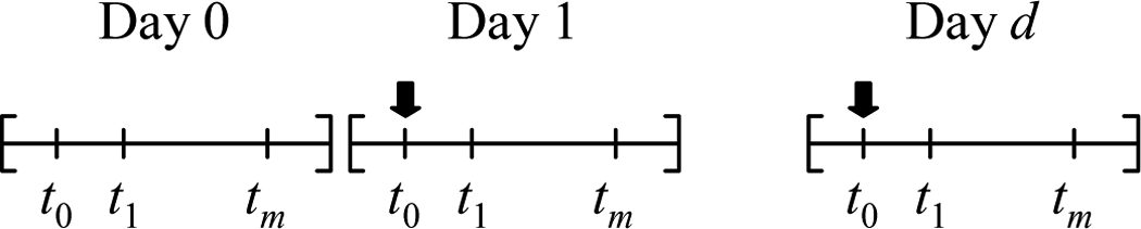 ZHANG ET AL.